Memo on lightGBM run on DNV data

In the gqc-utility-notebooks repo in the MSI machine, there is a gitignored data/ folder. It contains the utilized DNV data and the outputs from the notebooks pertaining to lightGBM.
Make sure the gqc-utility-notebooks virtual env is selected as the interpreter for the notebook.

tip

Refer the flow diagrams see the flow of events visually.

tip

From Q&A
Pavan: What are the best model types identified by the research on random tree based methods?

Vannary: LightGBM with oversampling (SMOTE) method is the best for I&I models for both utilities, and lightGBM with class weight is the best for structural models for both utilities.

01_GIS+Prediction_DNV_mapping_defects_version_2.ipynb

note

This reads in different DNV datasets separately and process them.

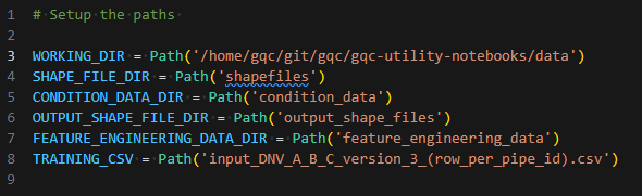
1. The default input / output paths are pointing to this data/ directory.

   WORKING_DIR = Path('/home/gqc/git/gqc/gqc-utility-notebooks/data')
   SHAPE_FILE_DIR = Path('shapefiles')
   CONDITION_DATA_DIR = Path('condition_data')
   
   OUTPUT_SHAPE_FILE_DIR = Path('output_shape_files')
   FEATURE_ENGINEERING_DATA_DIR = Path('feature_engineering_data')

2. Inputs

   Shapefiles:
   

   • SanFitting : Might be pipe fittings

   • SanHistMain: Historical pipe data

   • SanMain: Pipe data

     Condition data:
     
     

     Video lists:
     

3. Outputs

   Inspection info:
   

   Shape files with defects:
   
   There will be a group of files like: DNV_81_pacp_code_points.cpg DNV_81_pacp_code_points.dbf DNV_81_pacp_code_points.prj DNV_81_pacp_code_points.shp DNV_81_pacp_code_points.shx

4. Running the notebook:

   1. Run all cells up upto start here section and run start here.
   2. Run time is less than 1 minute for all cells.
   3. The output shape files can be downloaded from MSI machine to your windows machine and can be opened up in QGIS. (by dragging and dropping into a new QGIS window)

02_GIS+Prediction_prepare_data_for_defect_prediction_version_2

note

This notebook combines the different DNV data into a single CSV file, input_DNV_A_B_C_version_3(row_per_pipe_id).csv

1. Input files
   
   
   

2. Output files
   

3. Running:

   1. Run all cells except the prepare csv section.
   2. Total run time is less than 2 minutes.

03_RandomForest_xgb_lgbm_catboost

tip

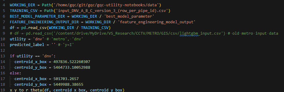
This only needs to be run one time for each new dataset to find and save the optimal model parameters. Saved parameters will be used in the next stages.

1. Input and output file paths and configuration
   

2. Running:

   1. Run everything before Run here section. Make sure the paths are correct in the Run here section.
   2. Select between I&I and structural defects through this line. y=I is I&I and anything else is structural defects

      predicted_label = '' # 'y=I'
   3. Run will be logged in to Weights and Biases in the CCTV_GIS_Prediction project. A link will appear in the first few lines of the output of the running cell.
   4. Last successful run took 5.5 hours to complete in the MSI machine.

04_GIS+Prediction_compile_results_CCTV_prediction_model

note

Not essential for production runs

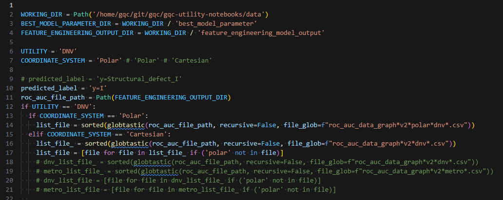
1. Input, output files, and configuration
   

2. Running:

   1. Check the configuration entires and run all cells.
   2. Runs in few minutes.

05_GIS+Predictions_generate_shap_plot

note

Not essential for production runs.

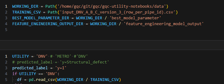
1. Input, output, and configuration.
   

2. Running:

   1. Check the configuration.
   2. Runs in around 10 minutes.

06_GIS+Predictions_save_the_predictions_to_shape_files

1. Input, output, and configuration
   
   

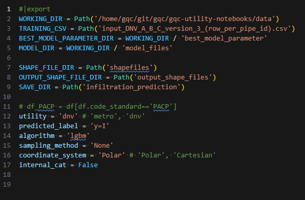
2. Running:

   1. Run all cells.
   2. Run time 50 min.